Designing Transforms for Data Reshaping with cdata

This note is about the design of data transforms using the cdata package. The cdata packages demonstrates the “coordinatized data” theory and includes an implementation of the “fluid data” methodology for general data re-shaping.

cdata adheres to the so-called “Rule of Representation”:

Fold knowledge into data, so program logic can be stupid and robust.

The Art of Unix Programming, Erick S. Raymond, Addison-Wesley, 2003

The design principle expressed by this rule is that it is much easier to reason about data than to try to reason about code, so using data to control your code is often a very good trade-off.

We showed in this article how cdata takes a transform control table to specify how you want your data reshaped. The question then becomes: how do you come up with the transform control table?

Let’s discuss that using the example from the article: “plotting the iris data faceted”.

The goal is to produce the following graph with ggplot2

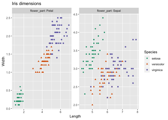
In order to do this, one wants data that looks like the following:

Notice Species is in a column so we can use it to choose colors. Also, flower_part is in a column so we can use it to facet.

However, iris data starts in the following format.

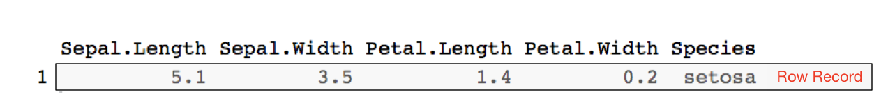
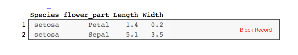
We call this form a row record because all the information about a single entity (a “record”) lies in a single row. When the information about an entity is distributed across several rows (in whatever shape), we call that a block record. So the goal is to transform the row records in iris into the desired block records before plotting.

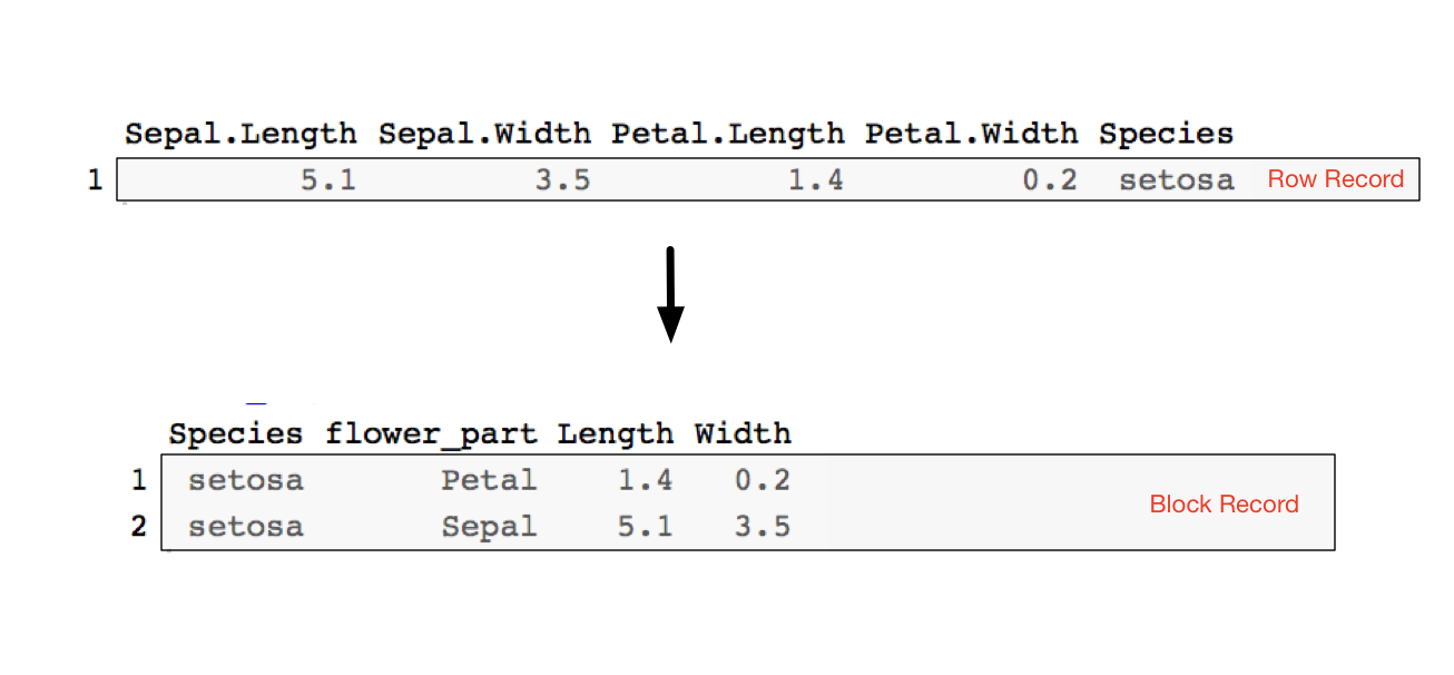
This new block record is partially keyed by the flower_part column, which tells us which piece of a record a row corresponds to (the petal information, or the sepal information). We could also add an iris_id as a per-record key; this we are not adding, as we do not need it for our graphing task. However, adding a per-record id makes the transform invertible, as is shown here.

There are a great number of ways to achieve the above transform. We are going to concentrate on the cdata methodology. We want to move data from an “all of the record is in one row” format to “the meaningful record unit is a block across several rows” format. In cdata this means we want to perform a rowrecs_to_blocks() transform. To do this we start by labeling the roles of different portion of the block oriented data example. In particular we identify:

Columns we want copied as additional row information (in this case Species, but often a per-record index or key).
The additional key that identifies parts of each multi-row record (in this case flower_part).
Levels we expect in the new record portion key column (Petal and Sepal).
New column names for the new data.frame. These will go where values are currently in the block record data.

We show this labeling below.

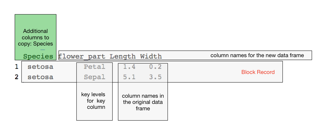
Notice we have marked the measurements 1.4, 0.2, 5.1, 3.5 as “column names”, not values. That is because we must show which columns in the original data frame these values are coming from.

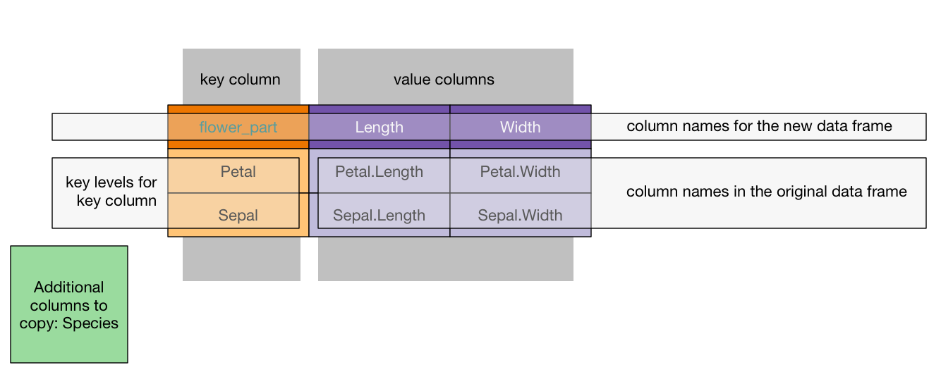
This annotated example record is the guide for building what we call the transform control table. We build up the transform control table following these rules:

The key column is the first column of the control table.
The key levels we wish to track are values in the key column.
The column names of the control table are the new column names we will produce in our result.
The block of values seen in our example record are replaced by the names of the columns that these values were taken from in the original data.
Any other columns we want copied are specified in the columnsToCopy argument.

The R version of the above is specified as follows:

# get a small sample of irises
iris <- head(iris, n = 3)
# add a record id to iris
iris$iris_id <- seq_len(nrow(iris))

knitr::kable(iris)

Sepal.Length	Sepal.Width	Petal.Length	Petal.Width	Species	iris_id
5.1	3.5	1.4	0.2	setosa	1
4.9	3.0	1.4	0.2	setosa	2
4.7	3.2	1.3	0.2	setosa	3

Specify the layout transform.

library("cdata")
#> Loading required package: wrapr

controlTable <- wrapr::qchar_frame(
  "flower_part", "Length"    , "Width"     |
  "Petal"      , Petal.Length, Petal.Width |
  "Sepal"      , Sepal.Length, Sepal.Width )

layout <- rowrecs_to_blocks_spec(
  controlTable,
  recordKeys = c("iris_id", "Species"))

print(layout)
#> {
#>  row_record <- wrapr::qchar_frame(
#>    "iris_id"  , "Species", "Petal.Length", "Petal.Width", "Sepal.Length", "Sepal.Width" |
#>      .        , .        , Petal.Length  , Petal.Width  , Sepal.Length  , Sepal.Width   )
#>  row_keys <- c('iris_id', 'Species')
#> 
#>  # becomes
#> 
#>  block_record <- wrapr::qchar_frame(
#>    "iris_id"  , "Species", "flower_part", "Length"    , "Width"     |
#>      .        , .        , "Petal"      , Petal.Length, Petal.Width |
#>      .        , .        , "Sepal"      , Sepal.Length, Sepal.Width )
#>  block_keys <- c('iris_id', 'Species', 'flower_part')
#> 
#>  # args: c(checkNames = TRUE, checkKeys = FALSE, strict = FALSE, allow_rqdatatable = FALSE)
#> }

And we can now perform the transform.

iris %.>%
  knitr::kable(.)

Sepal.Length	Sepal.Width	Petal.Length	Petal.Width	Species	iris_id
5.1	3.5	1.4	0.2	setosa	1
4.9	3.0	1.4	0.2	setosa	2
4.7	3.2	1.3	0.2	setosa	3

  
iris_aug <- iris %.>% 
  layout

iris_aug %.>%
  knitr::kable(.)

iris_id	Species	flower_part	Length	Width
1	setosa	Petal	1.4	0.2
1	setosa	Sepal	5.1	3.5
2	setosa	Petal	1.4	0.2
2	setosa	Sepal	4.9	3.0
3	setosa	Petal	1.3	0.2
3	setosa	Sepal	4.7	3.2

The data is now ready to plot using ggplot2 as was shown here.

Designing a blocks_to_rowrecs transform is just as easy, as the controlTable has the same shape as the incoming record block (assuming the record partial key controlling column is the first column). All one has to is get the reverse specification using t().

For example:

inv_layout <- t(layout)

print(inv_layout)
#> {
#>  block_record <- wrapr::qchar_frame(
#>    "iris_id"  , "Species", "flower_part", "Length"    , "Width"     |
#>      .        , .        , "Petal"      , Petal.Length, Petal.Width |
#>      .        , .        , "Sepal"      , Sepal.Length, Sepal.Width )
#>  block_keys <- c('iris_id', 'Species', 'flower_part')
#> 
#>  # becomes
#> 
#>  row_record <- wrapr::qchar_frame(
#>    "iris_id"  , "Species", "Petal.Length", "Petal.Width", "Sepal.Length", "Sepal.Width" |
#>      .        , .        , Petal.Length  , Petal.Width  , Sepal.Length  , Sepal.Width   )
#>  row_keys <- c('iris_id', 'Species')
#> 
#>  # args: c(checkNames = TRUE, checkKeys = FALSE, strict = FALSE, allow_rqdatatable = FALSE)
#> }

iris_aug %.>%
  inv_layout %.>%
  knitr::kable(.)

iris_id	Species	Petal.Length	Petal.Width	Sepal.Length	Sepal.Width
1	setosa	1.4	0.2	5.1	3.5
2	setosa	1.4	0.2	4.9	3.0
3	setosa	1.3	0.2	4.7	3.2

Notice in both cases that having examples of the before and after form of the transform is the guide to building the transform specification, that is, the transform control table. In practice: we highly recommend looking at your data, writing down what a single record on each side of the transform would look like, and then using that to fill out the control table on paper.

The exercise of designing a control table really opens your eyes to how data is moving in such transforms and exposes a lot of structure of data transforms. For example:

If the control table has two columns (one key column, one value column) then the operation could be implemented as a single tidyr gather() or spread().
If the control table has k rows then the rowrecs_to_blocks() direction could be implemented as k-1 rbind()s.

Some discussion of the nature of block records and row records in cdata can be found here.

Some additional tutorials on cdata data transforms can are given below:

John Mount, Nina Zumel

2021-06-11