rquery Introduction
John Mount, Win-Vector LLC
2022-01-22
Source:vignettes/rquery_intro.Rmd
rquery_intro.RmdIntroduction
rquery is a query generator for R. It is based on Edgar F. Codd’s relational algebra plus experience using SQL and dplyr at big data scale. The design represents an attempt to make SQL more teachable by denoting composition by a sequential pipeline notation instead of nested queries or functions. The implementation delivers reliable high performance data processing on large data systems such as Spark and databases. Package features include: data processing trees or pipelines as observable objects (able to report both columns produced and columns used), optimized SQL generation as an explicit user visible modeling step, convenience methods for applying query trees to in-memory data.frames, and low direct package dependencies.
Let’s set up our environment so we can work with examples.
run_vignette <- requireNamespace("DBI", quietly = TRUE) &&
requireNamespace("RSQLite", quietly = TRUE)## Loading required package: wrapr
# example database connection
db <- DBI::dbConnect(RSQLite::SQLite(),
                     ":memory:")
RSQLite::initExtension(db)

# adapt to database
dbopts <- rq_connection_tests(db)
options(dbopts)

# register database
old_o <- options(list("rquery.rquery_db_executor" = list(db = db)))
Table descriptions
rquery table descriptions are simple objects that store only the name of a table and expected columns. Any local data or database table that has at least the set of columns named in the table description can be used in a given rquery pipeline.
# copy in example data
rq_copy_to(
  db, 'd',
  data.frame(v = c(1, -5, 3)),
  temporary = FALSE,
  overwrite = TRUE)
## [1] "mk_td(\"d\", c( \"v\"))"
## v
## 1 1
## 2 -5
## 3 3
# produce a hande to existing table
d <- db_td(db, "d")
The table description “d” we have been using in examples was produced as a result of moving data to a database by rq_copy_to(). However we can also create a description of an existing database table with db_td() or even build a description by hand with mk_td(). Also one can build descriptions of local or in-memory data.frames with local_td().
Operators
The sql_node() alone can make writing, understanding, and maintaining complex data transformations as queries easier. And this node is a good introduction to some of the power of the rquery package. However, the primary purpose of rquery is to provide ready-made relational operators to further simplify to the point of rarely needing to use the sql_node() directly.
The primary operators supplied by rquery are:
The primary relational operators include:
-
extend()/extend_se(). Extend adds derived columns to a relation table. With a sufficiently powerfulSQLprovider this includes ordered and partitioned window functions. This operator also includes built-inseplyr-style assignment partitioning. -
project(). Project is usually portrayed as the equivalent to column selection, though the original definition includes aggregation. In our opinion the original relational nature of the operator is best captured by movingSQL’s “GROUP BY” aggregation functionality. -
natural_join(). This a specialized relational join operator, using all common columns as an equi-join condition. -
theta_join(). This is the relational join operator allowing an arbitrary predicate. -
select_rows(). This is Codd’s relational row selection. Obviouslyselectalone is an over-used and now ambiguous term (for example: it is already used as the “doit” verb inSQLand the column selector indplyr). -
rename_columns(). This operator renames sets of columns.
The primary non-relational (traditional SQL) operators are:
-
select_columns(). This allows choice of columns (central toSQL), but is not a relational operator as it can damage row-uniqueness. -
orderby(). Row order is not a concept in the relational algebra (and also not maintained in mostSQLimplementations). This operator is only useful when used with itslimit=option, or as the last step as data comes out of the relation store and is moved toR(where row-order is usually maintained).
The above list (and especially naming) are chosen to first match Codd’s relational concepts (project, select, rename, join, aggregation), SQL naming conventions. Notice this covers the primary dplyr operators mutate() (Codd’s extend), select() (not relational), filter() (Codd’s select, represented in SQL by “WHERE”), summarise() (Codd’s project or aggregate concepts, triggered in SQL by “GROUP BY”), arrange() (not a relational concept, implemented in SQL by “ORDER BY”). This correspondence is due to Codd’s ideas and SQL driving data engineering thinking for almost the last 50 years (both with and without credit or citation).
With relational operators the user can work fast and work further away from syntactic details. For example some R operators (such as is.na) are translated to SQL analogues (in this case IS NULL).
## SELECT
##  `v`,
##  ( CASE WHEN ( ( ( `v` ) IS NULL ) ) THEN ( 1 ) WHEN NOT ( ( ( `v` ) IS NULL ) ) THEN ( 0 ) ELSE NULL END )  AS `was_na`
## FROM (
##  SELECT
##   `v`
##  FROM
##   `d`
##  ) tsql_18797884537822469964_0000000000
The exact translation depends on the database (which is why to_sql() takes a database argument). Some care has to be taken as SQL types are different than R types (in particular for some databases logical types are not numeric).
With a database that supplies window functions one can quickly work the “logistic scoring by hand” example from
from Let’s Have Some Sympathy For The Part-time R User. This example worked with rquery code that works with both PostgreSQL and Spark can be found here.
We can demonstrate the pipeline, but the SQLite database we are using in this vignette does not have the window functions required to execute it. PostgreSQL, Spark, and many other databases do have the necessary functionality. The pipeline is a good example of a non-trivial sequence of relational nodes.
scale <- 0.237

dq <- mk_td("d3",
                   columns = qc(subjectID,
                                surveyCategory,
                                assessmentTotal)) %.>%
  extend(.,
             probability :=
               exp(assessmentTotal * scale))  %.>%
  normalize_cols(.,
                 "probability",
                 partitionby = 'subjectID') %.>%
  pick_top_k(.,
             partitionby = 'subjectID',
             orderby = c('probability', 'surveyCategory'),
             reverse = c('probability')) %.>%
  rename_columns(., 'diagnosis' := 'surveyCategory') %.>%
  select_columns(., c('subjectID',
                      'diagnosis',
                      'probability')) %.>%
  orderby(., 'subjectID')
qc() is “quoting concatenate”, a convenience function that lets us skip a few quote marks. No list(), as.name(), or quote() steps are needed as the operator nodes are parsed by R to find identifiers. The scale constant was added to the environment as pipelines try to bind constants during pipe construction (else scale would be estimated to be a missing column name).
Even though we are not going to run this query here, we can still check some properties of the query.
tables_used(dq)## [1] "d3"
columns_used(dq)## $d3
## [1] "subjectID" "surveyCategory" "assessmentTotal"
column_names(dq)## [1] "subjectID" "diagnosis" "probability"The operations can be printed as an operations tree.
## mk_td("d3", c(
##   "subjectID",
##   "surveyCategory",
##   "assessmentTotal")) %.>%
##  extend(.,
##   probability := exp(assessmentTotal * 0.237)) %.>%
##  extend(.,
##   probability := probability / sum(probability),
##   partitionby = c('subjectID'),
##   orderby = c(),
##   reverse = c()) %.>%
##  extend(.,
##   row_number := row_number(),
##   partitionby = c('subjectID'),
##   orderby = c('probability', 'surveyCategory'),
##   reverse = c('probability')) %.>%
##  select_rows(.,
##    row_number <= 1) %.>%
##  rename_columns(.,
##   c('diagnosis' = 'surveyCategory')) %.>%
##  select_columns(.,
##     c('subjectID', 'diagnosis', 'probability')) %.>%
##  order_rows(.,
##   c('subjectID'),
##   reverse = c(),
##   limit = NULL)
Notice the returned presentation is not exactly the set of nodes we specified. This is because of the nodes we used (normalize_cols() and pick_top_k()) are actually higher-order nodes (implemented in terms of nodes). Also extend() nodes are re-factored to be unambiguous in their use and re-use of column names.
We can also exhibit the SQL this operations tree renders, to (though the SQLite database we are using in vignettes does not have the required window-functions to execute it; we suggest using PostgreSQL).
## SELECT * FROM (
##  SELECT
##   `subjectID`,
##   `diagnosis`,
##   `probability`
##  FROM (
##   SELECT
##    `subjectID` AS `subjectID`,
##    `surveyCategory` AS `diagnosis`,
##    `probability` AS `probability`
##   FROM (
##    SELECT * FROM (
##     SELECT
##      `subjectID`,
##      `surveyCategory`,
##      `probability`,
##      row_number ( ) OVER (  PARTITION BY `subjectID` ORDER BY `probability` DESC, `surveyCategory` ) AS `row_number`
##     FROM (
##      SELECT
##       `subjectID`,
##       `surveyCategory`,
##       `probability` / sum ( `probability` ) OVER (  PARTITION BY `subjectID` ) AS `probability`
##      FROM (
##       SELECT
##        `subjectID`,
##        `surveyCategory`,
##        exp ( `assessmentTotal` * 0.237 )  AS `probability`
##       FROM (
##        SELECT
##         `subjectID`,
##         `surveyCategory`,
##         `assessmentTotal`
##        FROM
##         `d3`
##        ) tsql_19601181277043930904_0000000000
##       ) tsql_19601181277043930904_0000000001
##      ) tsql_19601181277043930904_0000000002
##    ) tsql_19601181277043930904_0000000003
##    WHERE `row_number` <= 1
##   ) tsql_19601181277043930904_0000000004
##  ) tsql_19601181277043930904_0000000005
## ) tsql_19601181277043930904_0000000006 ORDER BY `subjectID`
The above query is long, but actually quite performant.
To see the query executed, please see here.
Non-SQL nodes
Not all data transform steps can conveniently be written as a single SQL statement. To work around this potential limitation rquery supplies a special type of node called non_sql_node(). non_sql_node() is used to implement arbitrary table to table transforms as rquery pipeline steps. Two prototypical non_sql_node() is rsummary_node().
rsummary_node() builds a table of summary information about another database table. The format is each column of the original table produces a row of summary information in the result table. Here is a simple example.
d %.>%
  rsummary_node(.) %.>%
  execute(db, .)
## column index class nrows nna nunique min max mean sd lexmin
## 1 v 1 numeric 3 0 NA -5 3 -0.3333333 4.163332 NA
## lexmax
## 1 NAUsers can add additional capabilities by writing their own non_sql_node()s.
Standard interfaces
rquery goes out of its way to supply easy to program over value-oriented interfaces. For any meta-programming we suggest using wrapr::let(), a powerful and well-documented meta-programming system.
Assignment partitioning
rquery accepts many assignment in a sql_node() or in a single extend node. The extend node comes with automatic assignment partitioning to ensure correct and performant results. This allows the user to write large extend blocks and know they will be executed correctly.
Here is an example.
ot <- mk_td('d4',
                   columns = qc('a', 'b', 'c', 'd')) %.>%
  extend(.,
             x = a + 1,
             y = x + 1,
             u = b + 1,
             v = c + 1,
             w = d + 1)

cat(format(ot))
## mk_td("d4", c(
## "a",
## "b",
## "c",
## "d")) %.>%
## extend(.,
## x := a + 1,
## u := b + 1,
## v := c + 1,
## w := d + 1) %.>%
## extend(.,
## y := x + 1)Notice the dependent assignment was moved into its own extend block. This sort of transform is critical in getting correct results from SQL (here is an example of what can happen when one does not correctly mitigate this issue).
A node that uses the assignment partitioning and re-ordering is the if_else_block() which can be used to simulate block-oriented if-else semantics as seen in systems such as SAS (also meaning rquery can be critical porting code from SAS to SQL based R). This allows coordinated assignments such as the following:
ifet <- mk_td("d5",
                     columns = "test") %.>%
  extend_se(.,
            c(qae(x = '',
                  y = ''),
              if_else_block(
                qe(test > 5),
                thenexprs = qae(x = 'a',
                                y = 'b'),
                elseexprs = qae(x = 'b',
                                y = 'a')
              )))
cat(format(ifet))
## mk_td("d5", c(
## "test")) %.>%
## extend(.,
## x := "",
## y := "",
## ifebtest_1 := test > 5) %.>%
## extend(.,
## x := ifelse(ifebtest_1, "a", x),
## y := ifelse(ifebtest_1, "b", y)) %.>%
## extend(.,
## x := ifelse(!(ifebtest_1), "b", x),
## y := ifelse(!(ifebtest_1), "a", y))As you can see, the if_else_block() works by landing the test in a column and then using that column to conditional all further statements. qe() and qae() are quoting convenience functions. Note the if_else_block depends on x and y being defined before entering the block, as they are self-assigned ( this is checked by the extend node). The if_else_block() returns a list of assignments, which then used in the extend_se() statement, which in turn is re-factored into a sequence of safe extend nodes.
Performance
As rquery pipelines are factored into stages similar to the common relational operators they tend to be very compatible with downstream query optimizers. We think some of the advantage is the fact that rquery deliberately does not have a group_by operator, but instead considers this as the partitionby attribute of a project() node (non-trivial example here).
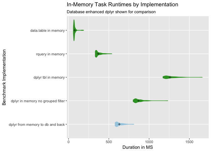
We have seen database based rquery outperform both in-memory dplyr and database based dplyr
(Figure from: here.)
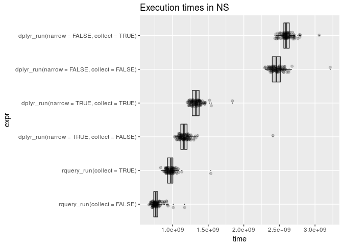
In addition rquery includes automatic column narrowing: where only columns used to construct the final result are pulled from initial tables. This feature is important in production (where data marts can be quite wide) and has show significant additional performance advantages
From a coding point of view the automatic narrowing effect looks like this.
wp <- mk_td(table = 'd6',
                   columns = letters[1:5]) %.>%
  extend(., res := a + b)

# full query
cat(to_sql(wp, db))
## SELECT
## `a`,
## `b`,
## `c`,
## `d`,
## `e`,
## `a` + `b` AS `res`
## FROM (
## SELECT
## `a`,
## `b`,
## `c`,
## `d`,
## `e`
## FROM
## `d6`
## ) tsql_52481097235700302167_0000000000
# longer pipeline
wn <- wp %.>%
  select_columns(., "res")

# notice select at end of the pipeline automatically
# gets propagated back to the beginning of the
# pipeline
cat(to_sql(wn, db))
## SELECT
## `res`
## FROM (
## SELECT
## `a` + `b` AS `res`
## FROM (
## SELECT
## `a`,
## `b`
## FROM
## `d6`
## ) tsql_23518476501118515504_0000000000
## ) tsql_23518476501118515504_0000000001A graph of the the effects of this kind of narrowing (for dplyr by hand as dplyr currently does not have the above type of automatic query analysis/optimization) shows the sensitivity to this optimization.
Conclusion
rquery is new package, but it is already proving to be correct (avoiding known data processing issues) and performant. For working with R at a big data scale (say using PostgreSQL or Spark) rquery is the right specialized tool for specifying data manipulation.
See also
For deeper dives into specific topics, please see also:
rquery README- Join Controller
- Join Dependency Sorting
- PerfTest
- Assignment Partitioner
- DifferentDBs
data.table basedimplementation
Appendix: Always clean up on the way out
options(old_o)
DBI::dbDisconnect(db)