Segmentation

John Mount

2020-12-15

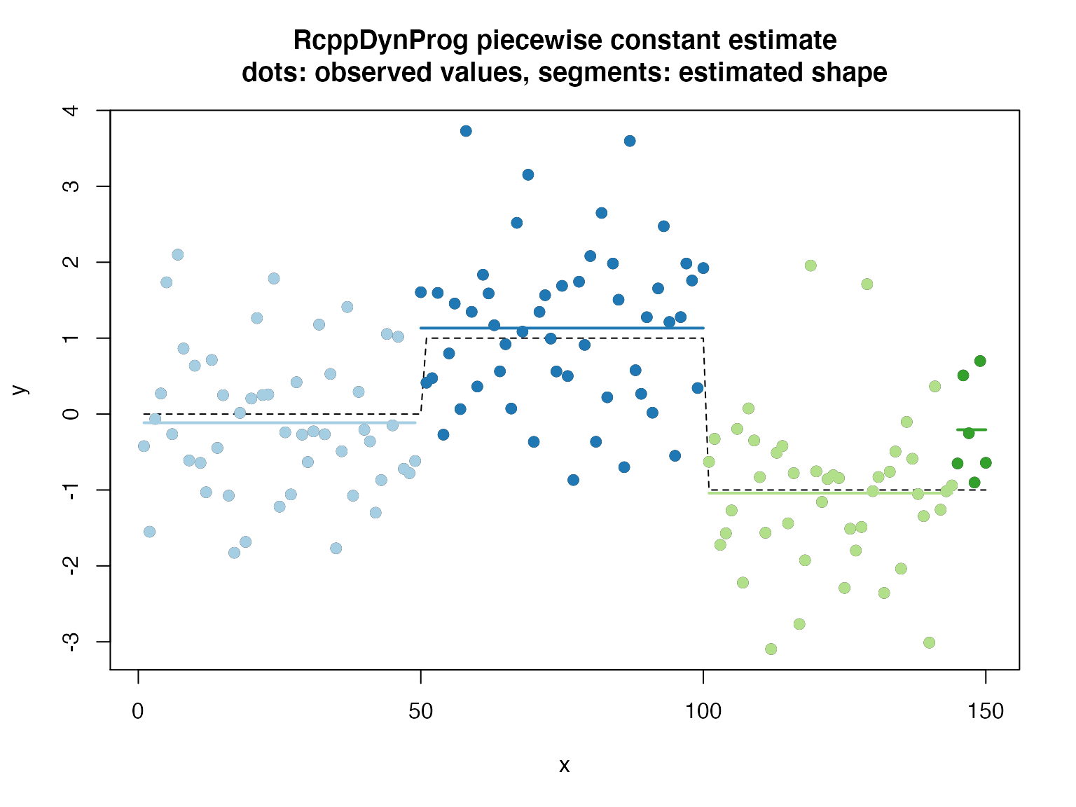
In this example we fit a piecewise constant function to example data.
Please see here for a discussion of the methodology.

library("RcppDynProg")


set.seed(2018)
g <- 50
d <- data.frame(
  x = 1:(3*g)) # ordered in x
d$y_ideal <- c(rep(0, g), rep(1, g), rep(-1, g))
d$y_observed <- d$y_ideal + rnorm(length(d$y_ideal))



# plot
plot(d$x, d$y_observed,
     xlab = "x", ylab = "y",
     main = "raw data\ncircles: observed values, dashed line: unobserved true values")
lines(d$x, d$y_ideal,
     type = "l",
     lty = "dashed")

As a heuristic, we set our regularization penalty to a value that treats permuted data (no relation between x and y) as a single partition.

y_permuted <- d$y_ideal[sample.int(nrow(d), nrow(d), replace = FALSE)]


solve_with_penalty <- function(ycol, penalty) {
  n <- length(ycol)
  indices = seq_len(n)
  x <- const_costs(ycol, 1+numeric(n), 1, indices)
  x <- x + penalty
  solve_interval_partition(x, n)
}

lb <- 1
ub <- 10
while(length(solve_with_penalty(y_permuted, ub))>2) {
  ub <- ub*2
}
while(TRUE) {
  mid <- ceiling((ub+lb)/2)
  if(mid>=ub) {
    break
  }
  si <- solve_with_penalty(y_permuted, mid)
  if(length(si)<=2) {
    ub <- mid
  } else {
    lb <- mid
  }
}
print(ub)

## [1] 2

We now use this penalty to segment the data. Notice we recover the actual problem structure.

soln <- solve_with_penalty(d$y_observed, ub)
print(soln)

## [1]   1  50 101 145 151

d$group <- as.character(findInterval(d$x, soln))
group_means <- tapply(d$y_observed, d$group, mean)
d$group_mean <- group_means[d$group]
d$estimate <- d$group_mean

print(sum((d$y_observed - d$y_ideal)^2))

## [1] 151.876

print(sum((d$group_mean - d$y_ideal)^2))

## [1] 6.653456

# plot
d$group <- as.character(d$group)
plot(d$x, d$y_observed,
     xlab = "x", ylab = "y",
     main = "RcppDynProg piecewise linear estimate\ndots: observed values, segments: estimated shape")
points(d$x, d$y_ideal,
     type = "l",
     lty = "dashed")
cmap <- c("#a6cee3",
          "#1f78b4",
          "#b2df8a",
          "#33a02c",
          "#fb9a99",
          "#e31a1c",
          "#fdbf6f",
          "#ff7f00",
          "#cab2d6",
          "#6a3d9a",
          "#ffff99",
          "#b15928")
names(cmap) <- as.character(seq_len(length(cmap)))
points(d$x, d$y_observed, col = cmap[d$group], pch=19)
groups <- sort(unique(d$group))
for(gi in groups) {
  di <- d[d$group==gi, , drop = FALSE]
  lines(di$x, di$estimate, col = cmap[di$group[[1]]], lwd=2)
}

The same solution through the more succinct solve_for_partitionc() interface.

# x_cuts <- solve_for_partition(d$x, d$y_observed)
# sometimes a different penalty due to problem chunking
x_cuts <- solve_for_partitionc(d$x, d$y_observed, penalty = ub)
print(x_cuts)

##     x       pred group  what
## 1   1 -0.1147501     1  left
## 2  49 -0.1147501     1 right
## 3  50  1.1321951     2  left
## 4 100  1.1321951     2 right
## 5 101 -1.0414092     3  left
## 6 144 -1.0414092     3 right
## 7 145 -0.2065736     4  left
## 8 150 -0.2065736     4 right

d$estimate <- approx(x_cuts$x, x_cuts$pred, xout = d$x, method = "constant", rule = 2)$y
d$group <- as.character(findInterval(d$x, x_cuts[x_cuts$what=="left", "x"]))

print(sum((d$y_observed - d$y_ideal)^2))

## [1] 151.876

print(sum((d$estimate - d$y_ideal)^2))

## [1] 6.653456

print(sum((d$estimate - d$y_observed)^2))

## [1] 144.2765

# plot
d$group <- as.character(d$group)
plot(d$x, d$y_observed,
     xlab = "x", ylab = "y",
     main = "RcppDynProg piecewise constant estimate\ndots: observed values, segments: estimated shape")
points(d$x, d$y_ideal,
     type = "l",
     lty = "dashed")
cmap <- c("#a6cee3",
          "#1f78b4",
          "#b2df8a",
          "#33a02c",
          "#fb9a99",
          "#e31a1c",
          "#fdbf6f",
          "#ff7f00",
          "#cab2d6",
          "#6a3d9a",
          "#ffff99",
          "#b15928")
names(cmap) <- as.character(seq_len(length(cmap)))
points(d$x, d$y_observed, col = cmap[d$group], pch=19)
groups <- sort(unique(d$group))
for(gi in groups) {
  di <- d[d$group==gi, , drop = FALSE]
  lines(di$x, di$estimate, col = cmap[di$group[[1]]], lwd=2)
}