Plot the relationship between two metrics.

MetricPairPlot(
  frame,
  xvar,
  truthVar,
  title,
  ...,
  x_metric = "false_positive_rate",
  y_metric = "true_positive_rate",
  truth_target = TRUE,
  points_to_plot = NULL,
  linecolor = "black"
)

Arguments

frame	data frame to get values from
xvar	name of the independent (input or model) column in frame
truthVar	name of the column to be predicted
title	title to place on plot
...	no unnamed argument, added to force named binding of later arguments.
x_metric	metric to be plotted. See Details for the list of allowed metrics
y_metric	metric to be plotted. See Details for the list of allowed metrics
truth_target	truth value considered to be positive.
points_to_plot	how many data points to use for plotting. Defaults to NULL (all data)
linecolor	character: name of line color

Details

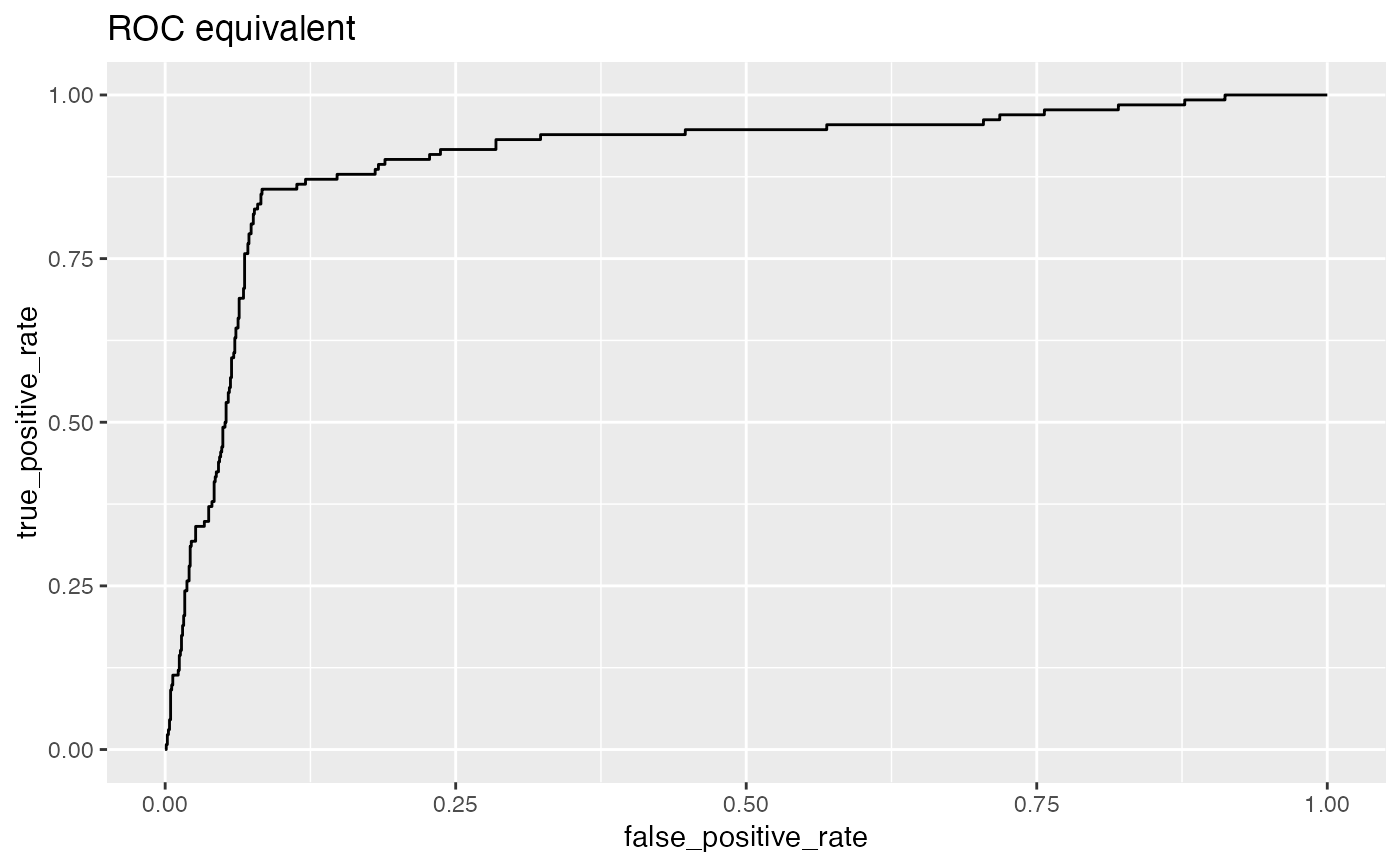
Plots two classifier metrics against each other, showing achievable combinations of performance metrics. For example, plotting true_positive_rate vs false_positive_rate recreates the ROC plot.

MetricPairPlot can plot a number of metrics. Some of the metrics are redundant, in keeping with the customary terminology of various analysis communities.

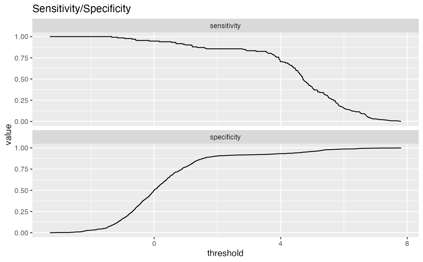
sensitivity: fraction of true positives that were predicted to be true (also known as the true positive rate)
specificity: fraction of true negatives to all negatives (or 1 - false_positive_rate)
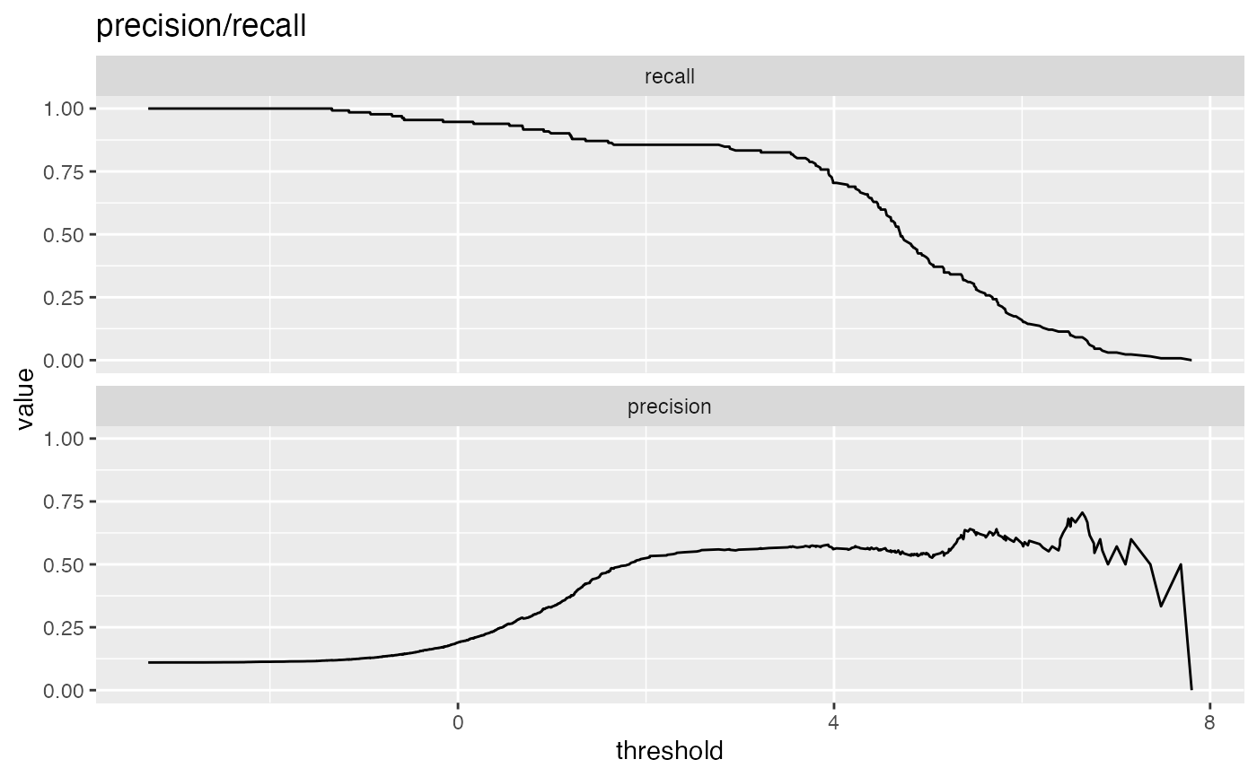
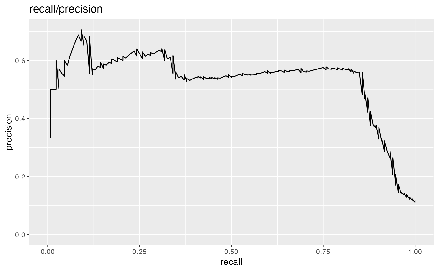
precision: fraction of predicted positives that are true positives
recall: same as sensitivity or true positive rate
accuracy: fraction of items correctly decided
false_positive_rate: fraction of negatives predicted to be true over all negatives
true_positive_rate: fraction of positives predicted to be true over all positives
false_negative_rate: fraction of positives predicted to be all false over all positives
true_negative_rate: fraction negatives predicted to be false over all negatives

points_to_plot specifies the approximate number of datums used to create the plots as an absolute count; for example setting points_to_plot = 200 uses approximately 200 points, rather than the entire data set. This can be useful when visualizing very large data sets.

Examples


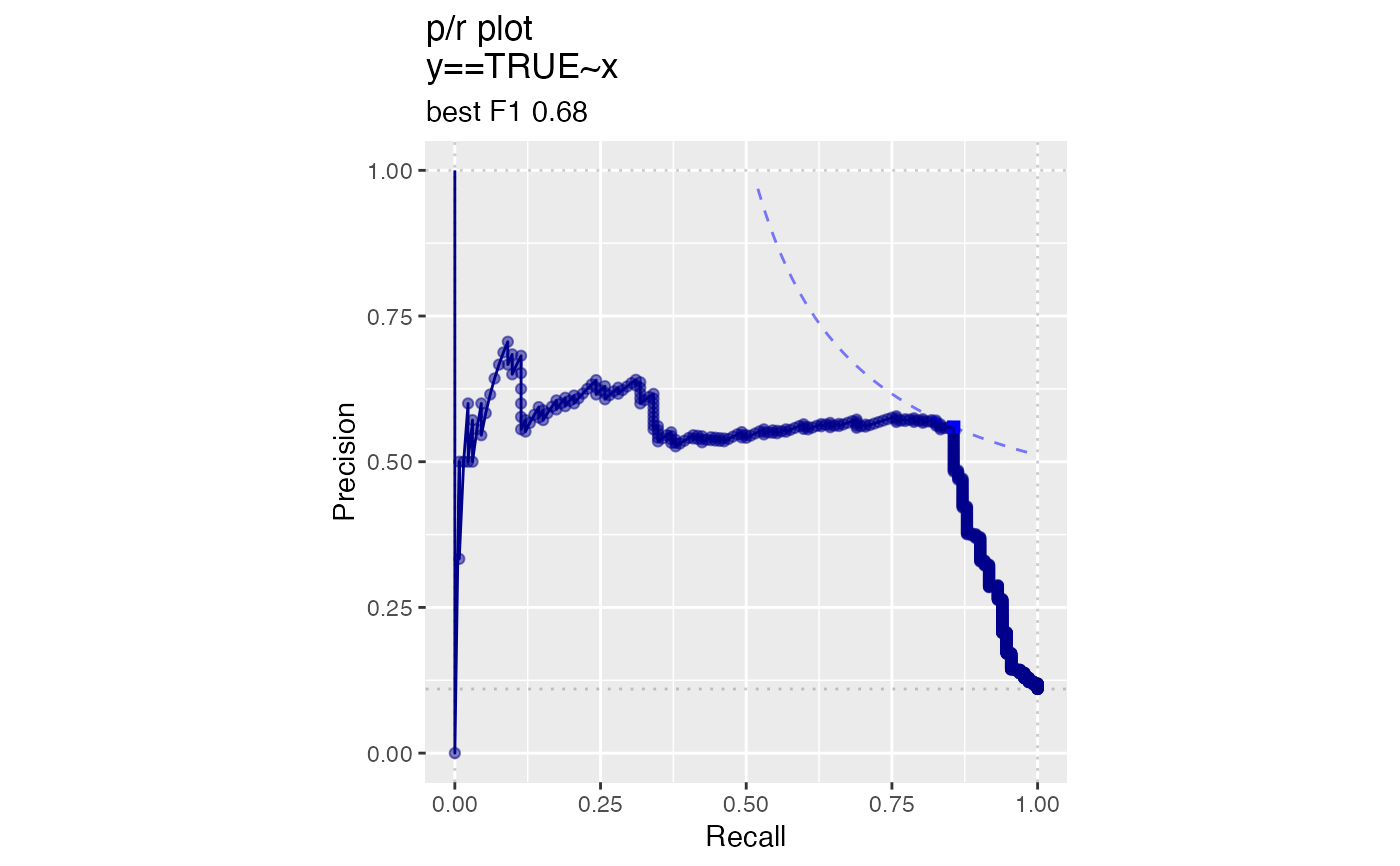
# data with two different regimes of behavior
d <- rbind(
  data.frame(
    x =  rnorm(1000),
    y = sample(c(TRUE, FALSE), prob = c(0.02, 0.98), size = 1000, replace = TRUE)),
  data.frame(
    x =  rnorm(200) + 5,
    y = sample(c(TRUE, FALSE), size = 200, replace = TRUE))
)

# Sensitivity/Specificity examples
ThresholdPlot(d, 'x', 'y',
   title = 'Sensitivity/Specificity',
   metrics = c('sensitivity', 'specificity'),
   truth_target = TRUE)
MetricPairPlot(d, 'x', 'y',
   x_metric = 'false_positive_rate',
   y_metric = 'true_positive_rate',
   truth_target = TRUE,
   title = 'ROC equivalent')
ROCPlot(d, 'x', 'y',
   truthTarget = TRUE,
   title = 'ROC example')

# Precision/Recall examples
ThresholdPlot(d, 'x', 'y',
   title = 'precision/recall',
   metrics = c('recall', 'precision'),
   truth_target = TRUE)
#> Warning: Removed 1 row(s) containing missing values (geom_path).
MetricPairPlot(d, 'x', 'y',
   x_metric = 'recall',
   y_metric = 'precision',
   title = 'recall/precision',
   truth_target = TRUE)
#> Warning: Removed 1 row(s) containing missing values (geom_path).
PRPlot(d, 'x', 'y',
   truthTarget = TRUE,
   title = 'p/r plot')

Plot the relationship between two metrics.

Arguments

Details

See also

Examples