Plot a Shadow Bar Plot

Plot a bar chart of row counts conditioned on the categorical variable condvar, faceted on a second categorical variable, refinevar. Each faceted plot also shows a "shadow plot" of the totals conditioned on condvar alone.

ShadowPlot(
  frm,
  condvar,
  refinevar,
  title,
  ...,
  monochrome = TRUE,
  palette = "Dark2",
  fillcolor = "darkblue",
  ncol = 1
)

Arguments

frm	data frame to get values from.
condvar	name of the primary conditioning variable (a categorical variable, controls x-axis).
refinevar	name of the second or refining conditioning variable (also a categorical variable, controls faceting).
title	title to place on plot.
...	no unnamed argument, added to force named binding of later arguments.
monochrome	logical: if TRUE, all facets filled with same color
palette	character: if monochrome==FALSE, name of brewer color palette (can be NULL)
fillcolor	character: if monochrome==TRUE, name of fill color for bars
ncol	numeric: number of columns in facet_wrap.

Value

a ggplot2 bar chart counting examples grouped by condvar, faceted by refinevar.

Details

This plot enables comparisons of subpopulation totals across both condvar and refinevar simultaneously.

By default, the facet plots are arranged in a single column. This can be changed with the optional ncol argument.

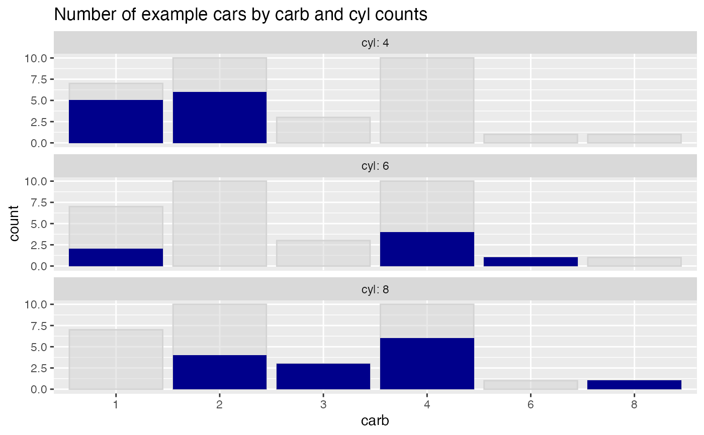
If palette is NULL, and monochrome is FALSE, plot colors will be chosen from the default ggplot2 palette. Setting palette to NULL allows the user to choose a non-Brewer palette, for example with scale_fill_manual. For consistency with previous releases, ShadowPlot defaults to monochrome = TRUE, while ShadowHist defaults to monochrome = FALSE.

Please see here for some interesting discussion https://drsimonj.svbtle.com/plotting-background-data-for-groups-with-ggplot2.

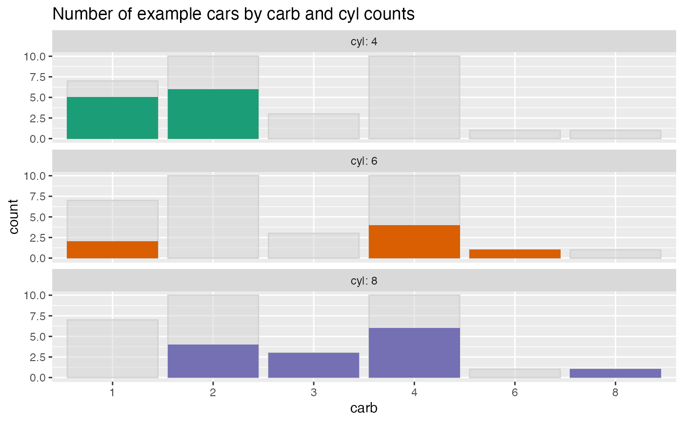
Examples

ShadowPlot(mtcars, "carb", "cyl",
           title = "Number of example cars by carb and cyl counts")

# colorcode the facets
ShadowPlot(mtcars, "carb", "cyl",
           monochrome = FALSE,
           title = "Number of example cars by carb and cyl counts")