Log-log plot — LogLogPlot • WVPlots

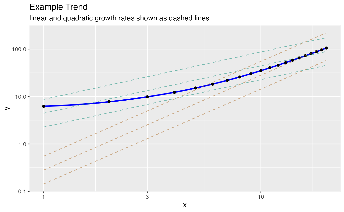
Plot a trend on log-log paper.

LogLogPlot(
  frame,
  xvar,
  yvar,
  title,
  ...,
  use_coord_trans = FALSE,
  point_color = "black",
  linear_color = "#018571",
  quadratic_color = "#a6611a",
  smoothing_color = "blue"
)

Arguments

frame	data frame to get values from
xvar	name of the independent (input or model) column in frame
yvar	name of the dependent (output or result to be modeled) column in frame
title	title to place on plot
...	no unnamed argument, added to force named binding of later arguments.
use_coord_trans	logical if TRUE, use coord_trans instead of `coord_trans(x = "log10", y = "log10")` instead of `scale_x_log10() + scale_y_log10()` (useful when there is not enough range to show ticks).
point_color	the color of the data points
linear_color	the color of the linear growth lines
quadratic_color	the color of the quadratic growth lines
smoothing_color	the color of the smoothing line through the data

Details

This plot is intended for plotting functions that are observed costs or durations as a function of problem size. In this case we expect the ideal or expected cost function to be non-decreasing. Any negative trends are assumed to arise from the noise model. The graph is specialized to compare non-decreasing linear and non-decreasing quadratic growth.

Some care must be taken in drawing conclusions from log-log plots, as the transform is fairly violent. Please see: "(Mar's Law) Everything is linear if plotted log-log with a fat magic marker" (from Akin's Laws of Spacecraft Design https://spacecraft.ssl.umd.edu/akins_laws.html), and "So You Think You Have a Power Law" http://bactra.org/weblog/491.html.

Examples


set.seed(5326)
frm = data.frame(x = 1:20)
frm$y <- 5 + frm$x + 0.2 * frm$x * frm$x + 0.1*abs(rnorm(nrow(frm)))
WVPlots::LogLogPlot(frm, "x", "y", title="Example Trend")
#> `geom_smooth()` using method = 'loess'