Plot a height scatter plot with marginals.

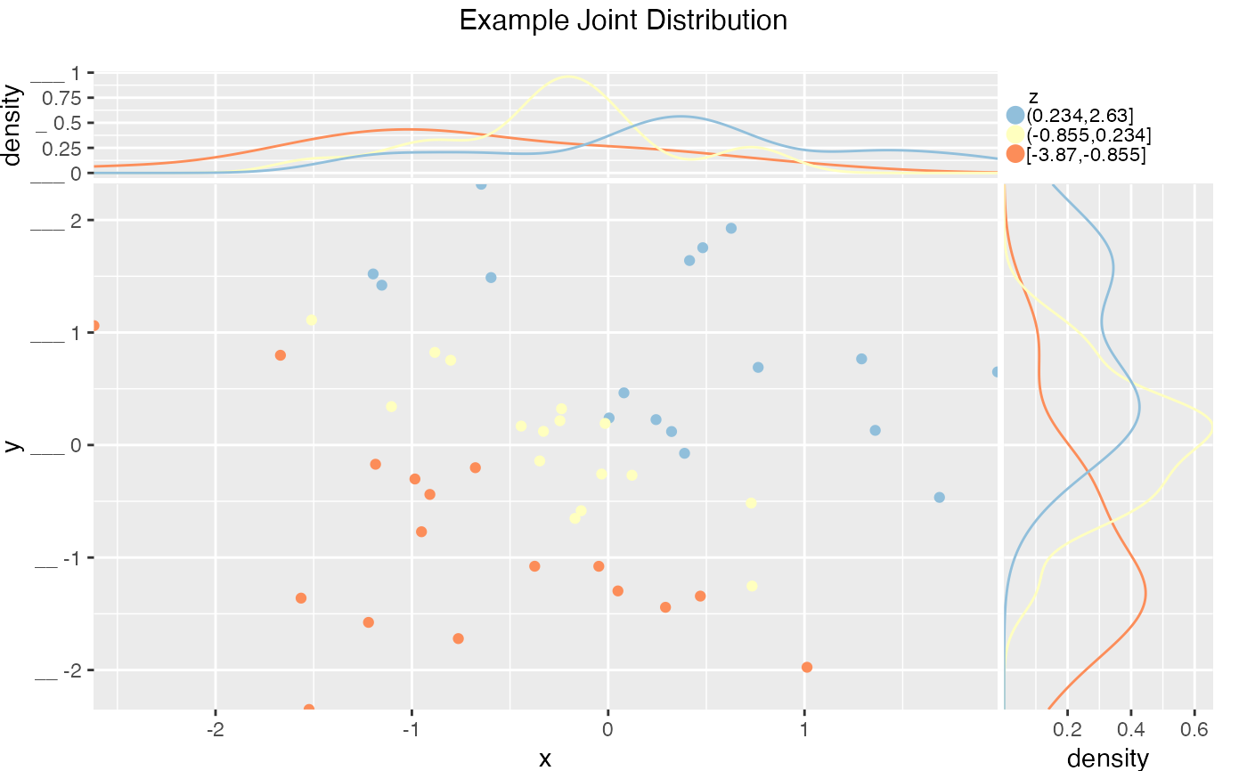
Plot a scatter plot conditioned on a continuous variable, with marginal conditional density plots.

ScatterHistN(
  frame,
  xvar,
  yvar,
  zvar,
  title,
  ...,
  annot_size = 3,
  colorPalette = "RdYlBu",
  nclus = 3,
  adjust_x = 1,
  adjust_y = 1
)

Arguments

frame	data frame to get values from
xvar	name of the x variable
yvar	name of the y variable
zvar	name of height variable
title	title to place on plot
...	no unnamed argument, added to force named binding of later arguments.
annot_size	numeric: scale annotation text (if present)
colorPalette	name of a Brewer palette (see https://colorbrewer2.org/ )
nclus	scalar: number of z-clusters to plot
adjust_x	numeric: adjust x density plot
adjust_y	numeric: adjust y density plot

Details

xvar and yvar are the coordinates of the points, and zvar is the continuous conditioning variable. zvar is partitioned into nclus disjoint ranges (by default, 3), which are then treated as discrete categories.The scatterplot and marginal density plots are color-coded by these categories.

See also

ScatterHistC

Examples

set.seed(34903490)
frm = data.frame(x=rnorm(50),y=rnorm(50))
frm$z <- frm$x+frm$y
WVPlots::ScatterHistN(frm, "x", "y", "z", title="Example Joint Distribution")